Today I want to talk a little bit about mental mill 1.2 - there are a couple of new features in the next version of mental mill that many of you will appreciate, since we heard requests for them over and over again. So we took the time to implement some of these.
New node types
There will be new node types in mental mill that can be recognized by their orange color. They are called "scene elements". There are several subtypes of scene elements. Even though all of them are equally important for the new workflow, the one you will be using most of the time is camera node.
A camera node inside mental mill displaying an entire scene built out of mutiple geometry using multiple shaders. All shaders are built with mental mill
Camera node
The camera node merges all your scene geometry into one view where you can render it using the realtime preview, mental ray or iray. You can also manipulate your scene: You can also select and move your lights and your geometry simply by clicking and dragging with the mouse.
A camera node may have its own environment attached to it. You may have any number of camera nodes in your workspace, each having its own environment shader attached.
A camera node with an environment shader attached. Each camera node may have its own environment shader which makes it practical for comparing multiple environment images.
Geometry nodes
For your scene to actually show some geometry, you need to create geometry nodes. There are two types: A geometry node that defines the type of geometry: There exists procedural shapes like the torus, sphere, plane and so on.
Various Geometry source nodes: Box, Terrain, .obj-file, Torus
The other geometry node actually defines the object in the scene. It must be fed by one of the aforementioned geometry nodes. Additionally it requires a shader connected to its 'material definition' input port. As soon as you have those set up, you have defined your geometry and it will be shown in the camera node.
Scene element being fed by a Texture_lookup_2d and a Geometry source node
Light nodes
You can create lights like any other scene elemnts using the context menu and creating a light. They use the same node types as geometry nodes, however, there are special ones that define the properties of the light source. Also, the scene element node that the light geometry is connected to also requires a light shader.
Scene Element being fed by a Light source node and a point light shader
You don't need to worry about wiring these scene elements manually - mental mill creates them automatically for you when you create them using the context menu.
Here is an example of a complete workspace in mental mill 1.2
Zoltan has created a very nice and elaborate tutorial about MetaSL based texturing in 3ds Max. Take a look and give it a try. During the series of articles, you will learn how to create this:
"This series of articles are about a texturing workflow and the related set of shader nodes called MUSH (MetaSL Utility Shaders). They allow the artist to texture up a mesh in high definition while keeping the artistic freedom to experiment and tweak the visuals in a simple way. These solutions are targeted mainly at game asset creators but might be useful to anyone who could live with the limitations of the methods."
- Zoltan
Here is a study of a water shader that I created a little while ago. The shader is based on a simple idea of using a black and white height map and a normal map that defines the heightmap where the water will be and how the normals are oriented.
See the screenshot of the shader network inside the Phenomenon. Many parts could be wrapped into Phenomena themselves, but I leave that to the users as a practice.
This is a preview of the water shader network inside the Phenomenon. I broke up the network into sections (though some functionalities overlap, but I tried to give it a rough structure. See the (Note that in the image one node does not belong to any section. This is because it does nothing, and I removed it from the final .xmsl that you can download from the mental mill blog)
How the effect is created (a rough overview)
Two different procedural perlin noises are combined to a float2 that is biased around 0 so that the values vary between -1 and 1. These values are used for
texture coordinate distortion (for the fake-refraction texture lookup)
caustic generation
water normal generation
A height map and a normal map that are both derived from the same source are used. The height map is used to calculate the water-falloff and the normal map provides the normal of the shape that 'contains' the water which is used for the diffuse shading.
The height information is used to create the falloff of the water (when it fades to the water color). Caustics are generated by using a special shader that is fed by the procedural float2 value.
All effects are finally combined and composited: Reflection, (fake) refraction, water color, caustics to generate the final look of the surface.
What to improve
The next things that would be interesting to do is, to find a way to replace the procedural waves with some cheaper normal textures that would save a massive number of instructions. However, this would raise the question how the caustics are generated, since this is done in a special shader.
I have created a set of Phenomena that assist you in debugging Colors and float2 as well as float parameters. The float debugger is basically the same as built into mental mill, but you are encouraged to open the Phenomenon and study what's inside there. The details are all described in the entry on the forum. Feel free to disassemble the Phenomenon and pull it apart, enhance it or create your own flavors.
Especially the color debugger has been enhanced and has more options than the built-in color debugger. It is more readable than the color encoding of the built-in debugger.
Color debugger: Shows when colors are above or below a given limit in red and blue. Components can be turned on and off and the behavior for the color overlay can be toggled: Either ALL components must exceed in order to show a color overlay or it is enough that ANY component exceeds in order to show a red/blue overlay. The other outputs of the debugger Phenomenon show a compressed view of the colors and the luminance.
Float debugger: Works basically like the built-in preview window debugger, but shows colored overlays instead of just clamping or repeating the values.
float2 debugger: debugs float2 parameters and shows a colored overlay where values go beyong or below the min/max range. Additionally it outputs the length as a float value.
As mentioned in my older blog entries, IQ of the Spanish demo group RGBA is one of my CG heroes. I know hardly any people who can combine mathematical understanding and arts in a more beautiful way. This prod here is quite old, but I just knew the still-image (a 4K executable). Here is also an animation where you can see procedural graphics at the highest level in a beautiful fly-over.
Recently I started playing with ICE in Softimage, which is a wonderfull node based tool for creating your own deformers, particle simulations and much more. The workflow reminds me a lot of mental mill (and I have always been a huge fan of node based editing systems) so it was not hard to get some results pretty soon.
As I was playing around, I couldn't help thinking about creating a shader in mental mill that implements a neat effect that takes advantage of ICE in Softimage. This tutorial won't be about ICE, though I will roughly explain a few details and I intend to post the project that I created along with the modified shader.
1.1 Preparation:
First you need to create folders and set up default paths so that you won't end up with absolute path names in your work. This will save you lots of time later on. Absolute path names are the root of all evil as soon as you start moving your files between multiple machines...
Under C:\users\username\Autodesk\Softimage_2010\Application\ create a folder called "CgFX" and another folder called "fxtextures". These will be needed for storing your exported shader and your textures.
Copy the textures that you will be using in this tuorial under C:\users\username\Autodesk\Softimage_2010\Application\fxtexturesso that Softimage will be able to load them automatically
Make sure that the texture path is added to mental mill's texture paths. To add a mental mill texture path, go to "Edit > Preferences > Path". Under Texture click Edit and add the path to your textures. This has the effect, that mental mill won't store absolute file paths when you select a texture from that directory.
Adding a texture path in mental mill
2. Implementation Softimage
Let's start in Softimage where I implemented an effect that attracts geometry to other geometry. So how does it work?
The "magnetic skin" effect in Softimage
I got a piece of geometry that I want to deform and another geometry that I will refer to as "attractor" since it will attract the other geometry as it is moved closer to the target geometry that has the ice effect applied.
2.1 ICE Deformer
In my ICE tree I search for the nearest points on the attractor and I calculate the average value, so that I know to which position the point is attracted to.
B is calculated as average position of the 'N' nearest points to point A.
As the distance between A and B gets smaller, A will be 'warped' more and more towards B
The distance of the source point to the averaged target position is calculated. I was implementing a falloff using the square distance, which can be expressed as 1/(distance^2).
The shorter the distance, the more the point will be attracted as the result of that calculation gets bigger. I made sure that the result of that calculation does not exceed the range between 0 and 1 by using a clamp node. This allowed me to calculate the final position by lerping between the original position value and the averaged value that I calculated on the attractor.
2.2 ICE weight map
The next "challenge" if you like to say so was to write the values that had been calculated into a Colors at vertices map. The data from that map can then be sent over to the shader.
So first I created a Colors at Vertices Property (Model > Property > Color At Vertices Map) into which I wanted to write the data calculated by the
However, it is not possible to set data that needs to be processed 'per sample' from an output that was calculated per point.
When manipulating point-based data, it can't be written into sample based maps.
The workaround is to stor the data in a temprary set data node and writing it into the
Color At Vertices map (see image below)
To circumvent that problem I took a look around and I found the explanation in the XSIBase forum that I still visit regularly. The answer is to write the data in some temporary variables using the Set Data node.
Then, when writing into the Vertex Color map (which is sample based) the data can be retrieved using Get -> self.nodelocation and retrieving the data that we set which is then written into the Vertex Color.
Now when switching to constant display, you can see the 'weight' as a grayscale being interpolated between the vertices. So much for the work that needs to be done in XSI. Next we will take a closer look at the actual shader that we will create in mental mill.
Inspecting the Vertex Color Map in Softimage. The more the points are
attracted, the brighter they appear in the map
3. mental mill shader implementation
The goal of this tutorial is to get an understanding of how to use Softimage ICE and shaders that were built in mental mill. For the sake of simplicity I reduce the size of the mental mill project to use just as few nodes as necessary.
The idea for the effect is that the original transforms (or simply blends) into another surface as the attractor moves closer and closer. This transition effect is controlled by the grayscale map that we generated in our ICE tree above.
3.1 The mental mill network for the Phenomenon "Break_D_Ice"
We want to blend between two materials. In order to give that impression, we will mix two bump maps as well as two diffuse texture maps and feed them into an illumination node. I used an Illumination_phong node (D) here.
The mental mill shader network: Note, that I renamed the Texture lookup nodes for more clarity.
3.2 Working around the Color At Vertices map in mental mill
Right now we just got one problem to solve: Mental mill does not know about any Color At Vertices Map, so we need to create a stand-in shader node. (We will replace it manually after we have exported the shader and loaded in in Softimage). For the stand-in I created a texture_lookup_2d node (G). I loaded a texture with spherical transition from white to black which allows me to preview the transitions in mental mill.
3.3 It's a matter of blend: Mixing textures
I used the result of the stand-in texture lookup node to blend the diffuse map textures (A) and (H). Note that I am multiplying (B) the two diffuse textures (A) and (H) before mixing, so the asphalt texture is modulated with the cracks.
Then the textures are mixed (C) and fed into the Illumination Phong node for both diffuse and specular texture. The result of the Illumination Phong node is fed to the result output of the Phenomenon. Note: Typically you would have separate textures for the specular color, I just try to keep the example small...
The same kind of blending is done with the normal maps. mental mill 1.1 ships with a couple of utility Phenomena so that you don't need to create the most basic utilities on your own. I used the Dual bump mixer here (E). Again, the bump mix is controlled by the stand-in texture lookup node. Since the 'Bump Mix' parameter of the Dual Bump Mixer takes a float value, it's converted from a color to a float.
3.4 The interface parameters to control the effect
It's always a good practice to reduce the amount of interface parameters to a minimum. This has several reasons:
The less parameters you have, the easier it is to tweak the shader.
Parameters that are not exposed can be made constants by the shader compiler which can reduce instruction count of the shader.
Interface parameters of the Phenomenon
You can see in the screenshots which parameters I chose to expose. Feel free to expose the parameters that you consider relevant.
3.5 Exporting the shader for Softimage
Finally, select your Phenomenon that you created and export it for Softimage under "File > Export..." and then select Autodesk Softimage (CgFX) from the dropdown menu. The location where you save the file is important. In newer Softimage versions (I used 2010) you need to store the shader files in a dedicated directory from which they will be loaded automatically upon startup. C:\users\username\Autodesk\Softimage_2010\Application\CgFX. (I had to create the CgFX folder manually, it was not present.)
Give the shader a meaningful name, I chose to name it Ice_breaker which will be then stored as Ice_breaker.cgfx.
There are other places that you can store your shader in. Check "Loading Existing Effects Files in the Preset Manager" of your Softimage Manual.
4. Loading the shader in Softimage
Next we will load the shader in Softimage. The realtime shader framework has changed in the recent version of Softimage. In older versions of Softimage you were able to load shaders using dedicated HLSL and CgFX nodes.
In the new version all you need is to store the shader in a dedicated directory from whichthe shader will be loaded.
4.1 loading the shader
(Re)Start Softimage and open the Render Tree. If you stored the shader in the right directory, you can find your shader under the Realtime > CgFX category in the Render Tree.
Realtime shaders in mental mill
Just drag and drop the shader from there to workspace and it is ready to be used: The image clips are automatically created and connected to your shader. If you set up your texture paths correctly as described under "preparation", then the images will be found automatically and the shader will display correctly.
4.2 How to feed a Color At Vertices map to the shader
The next step is about hand-massaging the shadercode, so that we can feed the Color At Vertices Map that our ICE tree is generating to the exported mental mill shader. For that we need to edit the shader a little bit. To edit a shader in Softimage, right click the shader instance in the Render Tree or in the shader list and choose "Edit Shader" from the context menu. This will open the shader code editor.
4.2.1 Understanding Realtime Shaders: A quick overview For the next step, you need to understand the structure of an exported MetaSL shader, so I will give a rough outline how realtime shaders work:
A realtime shader takes a number of data that can be defined either per vertex or globally per frame. Per vertex data is fed to the shader via a vertex stream. The per-vertex data is first passed to the vertex shader which may transform the data (transforming the vertex positions by viewing matrices, etc...). Other data might be passed through to the fragment shader without modifying it, for example UV coordinates.
In your shader code that mental mill is exporting for you, you don't have to worry about these things: mental mill takes care to set up all necessary vertex stream variables. Once the vertex streams are set up correctly, the right data that you want to process is automatically passed to the shader. Examples for per vertex data are:
Texture coordinates
Vertex Position
Normal
When you export a shader for Softimage, 4 different texture spaces are supported. As you just learned, texture coordinates are passed as vertex streams. In our example we just require the first texture space. This leaves 3 vertex streams that we can 'hijack' (or abuse) to feed our own vertex stream data to the shader.
Softimage has a convenient interface that lets you assign any vertex data from Softimage to the vertex stream variables of a shader.
Assigning data from Softimage to stream-variables of the CgFX Shader
This is what we need to do to get this working:
In the shader code we will locate the texture lookup function of the stand-in node that was simulating the Color At Vertices Map. The variable that holds the result of the texture lookup of the stand-in node will be overwritten with the value that comes from the vertex stream variable that we 'hijacked'. That way you obtain the real value from the vertex stream data that the Ice Tree in Softimage is computing.
While that may sound like one daunting step it just requires a trivial change to the shader. Nevertheless I want you to understand what we are doing exactly and why we are doing this, so let me me explain:
When a mental mill shader is exported, all shader nodes are converted to functions in the exported shader code that will be called in the correct order to carry out all necessary tasks. In step 3.2 we created a stand-in texture lookup node that was acting as a holdout for our Color At Vertices map.
4.2.2 Editing the mental mill shader to use texture space slot for passthrough
As we just said: We want to use a texture space to pass the Color At Vertices information from Softimage to the shader. Lets take a look at the vertex shader that you exported from mental mill:
You can see, that the Vert2Frag structure holds an array of 4 vertex streams (in the image below on the left, colored in orange).
In the vertex shader this stream array is passed to the state-structure variable state.tex_coord, colored in green. We need to remember where this stream data is stored. The first array element stream will hold the texture coordinates that we will be using for the texture lookups. The second one will hold the Color at Vertices Data.
Now we need to find the Texture lookup and replace it with the variable that holds the result of the texture lookup with the vertex stream value.
Look for the main-function of the phenomenon that you exported from mental mill. In my case, the Phenomenon was called "Break_D_ice", so the function is called "Break_D_ice_main".
The stand-in texture lookup node was renamed to "Weightmap". Inside the "Break_D_ice_main" function you need to find the function call which is a combination of the Nodename in mental mill and some additional strings to avoid name collisions. In my case it was called "Break_D_Ice_Texture_lookup_main(...)". Above the variable that will hold the result, "float4 msl_Weightmap_result" is declared.
Comment out the texture lookup function.
When "float4 msl_Weightmap_result" is declared, assign it the texture stream variable: float4 msl_Weightmap_result = float4(state.tex_coord[1].xyz, 1);
In the Shader Code editor of Softimage click "Validate" to check your shader for errors. The shader should validate and you are ready to Apply it.
If you set up everything correctly, make sure that your viewport is set to "OpenGL" preview. Below you can see some examples. I tried to vary the effect a little bit more. you can make your mental mill example much more sophisticated by extending this example. So feel free to do so!
5 Conclusion
In this tutorial you learned some techniques that allow you to customize and hand tweak your shader code. It's important to understand that by knowing a little bit of Cg (or HLSL) you can start customizing your shader code so that it fits on top of almost any engine.
Also remember the way that data is passed to a shader. You saw, that in Softimage you can assign almost any data to a vertex stream. Knowing that, this allows you to add certain features by hand if you are familiar with your favorite DCC tool and CgFx/HLSL.
Here you can see a video clip how to export the shader from mental mill and load it in Softimage:
Further reading:
The CG Tutorial
This book that is available online gives you a better idea of how the CG language works and you can learn more about the structure of a cg shader.
Today I will talk about some unspoken secrets about navigating and resizing nodes in mental mill 1.1. The nodes in mental mill can be navigated and resized in a much more sophisticated way than most users might think, so I will share those secrets with you today!
Hiding input and output parameters
Hold down the shift-key and resize the top or the bottom of your node. This will conceal the input or ouput parameter section of a node.
Scrolling within a node that is partly concealed
When a node has been changed so that either parts of the input- or output parameter section are not visible, a light gray scroll bar appears on the side. For input parameters, the scroll bar will appear on the right side, output parameters can be scrolled on the right side.
Collapsing a node
You can collapse a node all the way: Hold the shift key and drag the top or bottom border of the node so that it is entirely collapsed . This is very useful when you have nodes on your workspace that don't play an important role and that you don't want to clutter up your view. If you have got any other nodes connected, you can see that the connection wires are made semi-transparent.
Scrolling a party collapsed node / Restoring a node
Double-click the Top or Bottom bar of a node to restore its default view.
You can use the scroll bars to scroll within an input or output parameter section that is partly concealed
When the node is in a semi-collapsed state, you can left-click and drag the splitter bar in the middle to hide and reveal the input parameter section.
Resizing preview windows
The preview windows of the output parameters of a node can be resized individually: Click and drag one of the corners of the preview window.
Preview windows can be opened and closed by left-clicking the name of the output parameter.
In the previous post I explained how you can create a ray pattern effect using basis mental mill nodes. This involved some math operations and it took a couple of nodes to make the effect work. We want to achieve the
same result in a simpler way, so next I show you how to use the curve nodes that come with mental mill curve shader pack.
This pack includes nodes that generate one dimensional curves which can be used to drive shader parameters, remap values and colors and generate textures and patterns.
When you use those curve nodes for the first time you might get the feeling that this whole concept is a bit abstract, so I would like to give you an idea of how versatile these shaders really are and I will show one use case.
Curve Shapes Curve shaders are able to generate curves of all kinds of shapes. Basically they implement a mathematical functions of the style y=f(x) which means that for a given input value X an output value Y is computed. The curve shader nodes were designed that you are able to see the curves graphically by opening the "graph_out" parameter of a curve node.
Curves can be used to generate patterns using the "gradient_linear" and "gradient_radial" nodes.
Here you can see which kinds of curves you can generate
Angular and radial gradient - the boolean
switch allows to change the generation behavior
Let's try that: Just attach a curve shader to the 'curve' input of the gradient_radial node. You can change the way that the pattern is generated by enabling the boolean parameter 'Circular' which will generate a circular pattern.
Try different curves and you see how the generated texture changes. If you want to create a fancy ray pattern, use the noise_1d curve which gives you a large number of animatable parameters to generate random looking rays.
Adding variation
Now you know how to generate basic patterns. It gets more interesting when you start sidechaining other gradient nodes which I will show in the next steps:
The gradient_radial node has an input parameter 'offset'. Create another gradient_radial node, convert it to a float value and attach it to the 'offset' parameter of the first gradient_radial node: You see that it generates a spiral now.
I guess now you know where we will be going with this example: The offset is now driven by another gradient node. So what happens if we attach another curve generator to the second gradient node? Let's try that:
You see that the offset is too strong and that it's only offsetting in one direction because we feed only positive values to the offset. So let's change the range using a Math_float_lerp node. (Remember: A lerp nodes interpolates incoming values that ramge from 0 to 1 to range from 'start' to 'end' so that 0 is mapped to 'start' and 1 is mapped to 'end'. Values outside that range are extrapolated. )
Now the offset gives some really interesting result which we can further elaborate on by animating it. So lets add some animation on top:
Create a state_animation_time and send it to a math_float_multiply so that you can adjust the speed of the animation. Connect the result to the offset parameter of the second generator node.
Start the animation now and see, how the ray pattern is animated now.
From there you get the idea how you can create arbitrarily complex patterns by combining several gradients that drive other gradients.
Conclusion: In case you need to create fancy ray patterns for some retro-70ies effect, you now know what you need. Though I'd expect you won't need to create this kind of procedural patterns too often, you get an idea of how you can use curve nodes to create different kinds of gradients. Driving one gradient with the result of another gradient node and adding animation on top allows you to create sophisticated effects. Curve nodes allow you to create much more interesting effects and there are more use cases - I intend to show more in another post. Have fun creating your own fancy patterns and playing around with them!
This time I assembled an example that shows how to create a kind of funky sunbeam-effect using the MetaSL shaders. I won't go too much into the details this time. I tried to make the project quite self-explaining. Just start at the top of the workspace where you can see some nodes connected. This is the basic idea of how the ray pattern is created. Further down in the workspace you can find several Phenomena that extend the ray pattern effect. Later I will show you how you can achieve the same effect much easier using the MetaSL curve shaders.
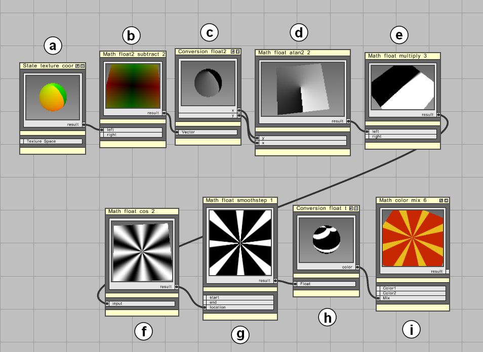
The texture space is offset so that it ranges from -0.5 to +0.5 (a and b). The u and v components are split (c) and then fed into a Math_float_atan2 (d) node. This returns values that range from -PI to +PI. By multiplying this with an integer (e) (well actually it is a float, i guess you know what I mean) and feeding it into a Math_float_cos node (f) you get a result that ranges from -1 to +1 and creates the ray pattern.
To shape the rays I used a Math_float_smoothstep (g) node. The result of the cosine-node is fed into the 'locaction' input of the Math_float_smoothstep node. For the input parameters 'start' and 'end' use values that are close to each other to get a crisper transition. Applicable ranges are between -1 and +1.
Finally the resulting float value is converted to a color (h) and fed into the mix parameter of a Math_color_mix node (i) that you can use to mix two different colors.
Next I will show you how to use the MetaSL curve shaders to achieve the same effect but faster and in a more versatile way.
Recently we have been at the GDC in San Francisco which has been a really great show. As usual we have been showing off mental mill at the NVidia booth where we were demoing the latest version of mental mill, namely an early version of 1.2.
Unfortunately my pocket camera did not work too well under the lighting conditions on the showfloor, so there are no good images to show, unfortunately. However, I got one shot of David explaining the software to an interested person.
We gave a preview of the new features that have been added to mental mill 1.2 and it was interesting to discuss with the users and hear their feedback. For those who have not been at the GDC, here are some of the highlights that we were showing:
scene element nodes: In version 1.2 there are new node types that describe a scene that can be previewed inside mental mill. These include the description of geometry, lights and a camera.
Load any number of preview objects and apply different shaders to them
View all geometry in one scene (which is practical if you have a model that is made out of several pieces of geometry that need different shaders)
Render previews with iray and mental ray directly inside the camera node on the workspace. No need to launch a separate render window.
Shader creation for iray: iray supports a subset of shaders that you can easily wire up in mental mill and render it with iray inside the camera node
Project manager: The project manager helps to keep an overview over the shader files and shaders used in your project which helps you to keep an overview over your shader assets.
For our demos we were kindly provided with models by The Game Assembly which has some talented artists that created some cool models. Thanks for their collaboration, I hope to post some images soon.
Today the the website www.metasl.org went online. For all those mental mill users who are interested in writing their own shaders, this is a comprehensive resource that helps to quickly get an idea of how to use MetaSL.
Right now the webpage is work in progress. For now you can find the first four chapters which are also available as PDF downloads for reading offline. These are draft versions of chapters and might be changed and updated.
New chapters will be added in the next weeks.
The chapters so far are:
Chapter 1: MetaSL — Strategy and scope
Chapter 2: Elements of the MetaSL language
Chapter 3: Basic surface shaders
Chapter 4: Rendering state
MetaSL is a platform independent shading language that can be translated to any existing target shading language. This makes it extremely useful if you need to deploy your shader on multiple platforms. Furthermore, you need to write your shader only once, allowing you to concentrate on the algorithmic aspect of your code rather than porting it manually from one language to another.
For sending feedback, you can take a look at the MetaSL Book open forum where you can leave your message and discuss with others.